Ordered Discrete Data

Ordered, discrete data is common, e.g.

{bad, poor, average, fair, good}, or

accident "rating" categories (for insurance), or

{fascist, conservative, liberal, left-wing, communist},

etc..

If the frequency counts for the categories are quite large, the data can be modelled successfully by a multi-state distribution.

If the frequency counts are small, i.e. the amount of data is small for the number of categories, the cost of stating all the parameters of an unconstrained multi-state distribution may be prohibitive. This can cause a problem, e.g. in decision trees where the amount of data arriving at a particular leaf can be small.

Best is to keep and make use of the fact that the data are ordered (class Ord in Haskell), discrete which can be used to advantage, e.g. in [partitioning] such data-spaces.

Priors

The key question is what prior should be placed on distributions for ordered discrete data, i.e. what kind of distribution should be favoured? It is clear that, given sufficiently convincing data, either (i) any favoured kind of distribution should tend to a (unordered) multi-state distribution or (ii) a multi-state distribution should become competitive (v. ordered).

Possible properties to be favoured apriori:

uni-modal,

smooth.

Unimodal

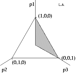
Given M categories, the largest probability is say T_i, 1<=i<M. Given that, T₁, ..., T_i-1 must be non-decreasing, and T_i+1, ..., T_M must be non-increasing.

e.g. M = 3, allowed:

T₁ >= T₂ >= T₃

T₂ >= T₁ >= T₃

T₂ >= T₃ >= T₁

T₃ >= T₂ >= T₁

i.e. 4 out of the 6 unconstrained 3-state distributions are allowed.

Message length

A reasonable approach is to code the parameters of a unimodal distribution by the method used for the (unconstrained) multi-state distribution. There is some slight inefficiency if the probabilities of two adjacent categories are close in value with respect to their uncertainties.

Normalisation: In general given M-states, the allowed fraction of acceptable distributions is

∑_i=1..M {(M-1)! / ((i-1)! . (M-i)!)} = 2^M-1 cases out of M! permutations.

i.e.

M	allowed	out of M!	saving	e.g. M=3
2	2	2	0 bits
3	4	6	.5 bits
4	8	24	1.5 bits
5	16	120	3 bits
6	32	720	5.5 bits
7	64	5040	6.5 bits

Saving = log₂(M!) - (M-1) bits

Note that M=5 to M=7 is typical survey-form territory.

Estimator (search)

There is unlikely to be a closed form for the MML estimator for a unimodal distribution. However a constrained search of the unimodal region should not be too difficult. A "smoothed" distribution derived from the obvious unconstrained M-state estimate may provide a good starting point.

The `uni1' code is based on counting frequencies of letters, from the left, while forcing the frequency counts to remain unimodal at all times. The `uni2' code is better, based on the unordered MML code, smoothed to make it unimodal if necessary. -- No claims to optimality; uni2 usually beats uni1, but rarely uni1 beats uni2 slightly, so neither is optimal in general.