A General Objective for Inductive Inference

C. S. Wallace & M. P. Georgeff
Technical Report No. 32
March 1983
Department of Computer Science, Monash University, Australia 3168

Abstract

In this paper we present a general framework for inductive inference. We define what constitutes an acceptable explanation of a body of data, and use the length of an explanation as a measure for selecting the best of a set of competing theories.

An explanation is defined to consist of two compatible parts, a binary string specifying the theory and another binary string specifying the degree of fit between the theory and the data. Examples are given from a wide range of fields which indicate how explanations are constructed and used to find optimal theories. Further, we show how the specification language for theories defines a prior probability distribution over families of models and a framework in which prior expectations about simple components of the model may be combined. Unlike previous attempts using a Bayesian approach, our technique also allows us to deal with continua of models.

1. Introduction

We address the problem of forming an hypothesis or theory by induction from a body of data, and propose a quantitative objective function which may be used to compare alternative theories or hypotheses about the same body of data in a very wide range of fields.

Informally, we consider an "explanation" of a body of data to consist of a message or symbol string comprising two parts. The first part is a statement of an hypothesis about the data, stated in some "appropriate" language. The second part is a coded representation of the data, using a code which would be optimal (in the sense of least expected length) were the stated hypothesis true. The objective function is the length of the explanation. Of two of more hypotheses from the data, that hypothesis yielding the shortest explanation is preferred.

We do not directly address the methods which might be used to infer good hypotheses from the data, except in the context of the specific examples discussed in the paper.

2. Explanations

Suppose we have a body of data D being the concatenation of one or more sentences in a language L₀. For simplicity we assume L₀, and all other strings and languages discussed, to be over a binary alphabet. Assume sentences in L₀ have the prefix property - no sentence is the prefix of another, hence the binary string D can unambiguously be decomposed into its constituent sentences. Further, if D is the concatenation of sentences D₁, D₂, ..., D_n, assume that each sentence represents an independent piece of data, so that any permutation of these sentences is also a valid representation of the data in L₀.

For a given deterministic Turing machine (TM) M₀, let <M₀>I be the output resulting from inputting string I to M₀. Then I is an explanation of D=D₁, D₂, ..., D_n with respect to M₀ iff

(a) <M₀>I = D

(b) I has the form I' I₁ I₂ ... I_n where for every sentence in D,  <M₀>I' I_j = D_j   (j = 1 ... n).

(c) len(I) < len(D)

If I and J are both explanations of D with respect to M₀, we say I is better than J with respect to M₀ if len(I) < len(J). Where no ambiguity arises, we will simply say I is better than J.

The above definition of an explanation is with respect to a given machine M₀. The following sections develop a formal description of M₀, without prejudicing the possible substantive choices of M₀.

3. Theories

We define a Probabilistic Turing Machine (PTM), M, as a Turing machine with a stochastic transition function. Let t_M(s,c) be the value of M's transition function while in state s and scanning tape symbol c. For each state s and symbol c, t_M(s,c) is a set of quadruples <s_i, c_i, d_i, p_i> called moves, where s_i is the next state, c_i is the symbol to be written, d_i is the direction of the tape movement, and p_i is the probability of the machine's making this move. The sum of p_i over all moves in t_M(s,c) is one, for all s and c.

A behaviour of M is any sequence of moves that can be made by M, beginning in the start state and ending when a final state is reached. The probability of a behaviour is the product of the probabilities of the moves in the sequence.

For each state s and tape symbol c, assign a unique label to each move in t_M(s,c). Then each behaviour of M can be described by a string of labels, called a control sentence of M. The set of such strings is called the control language of M, denoted C(M). (In language theory, C(M) is usually called the associated language of M (Salomaa 1973)).

We now describe a binary representation of the control language. For each state s and tape symbol c, the values of p_i in the set of moves t_M(s,c) form a discrete probability distribution over the set of moves. Construct a Huffman code over a binary alphabet optimised for this distribution. Then to each label there corresponds a binary code word of length ceiling(-log p_i), where p_i is the probability of the labelled move. Here and subsequently, logarithms are to base 2, and the rounding will be neglected. The binary control language BC(M) is derived from C(M) by replacing every label by its corresponding binary code word. Then BC(M) has the property that if w is a sentence in BC(M) encoding some behaviour of M the length or w is minus the logarithm of the probability of the behaviour. For w in BC(M), the output of behaviour w, written <M>:w, is the content of M's tape at the end of the behaviour.

Note that sentences of BC(M) have the prefix property. Note further that the optimality, in the sense of expected length, of Huffman codes ensures that of possible binary languages for describing the behaviour of M, BC(M) is among the most concise.

Let M be the (possibly infinite) set of PTMs described by sentences in a language L₁ with the prefix property. We write M_m to denote the machine described by a sentence m in L₁. We define M₀ to be a deterministic TM that takes a string m w₁ w₂ ... w_n, where m is a sentence in L₁ and w₁, w₂, ..., w_n are sentences in the binary control language of M_m, and produces the output string

<M_m>:w₁  <M_m>:w₂  ...  <M_m>:w_n

Thus, if I = I' I₁ I₂ ... I_n is an explanation of D = D₁ D₂ ... D_n with respect to M₀, we may equate

I' = m

I_j = w_j  and  D_j = <M_m'>:w_j (j = 1...n)

We then call m (or M_m) a theory about D, and say that m is better than m' with respect to M₀ if there exists w = w₁ w₂ ... w_n such that

<M_m>:w = D

and for all w' such that <M_m'>:w' = D,

len(m w) < len(m' w')

Informally, m nominates a PTM M_m which is a model of an hypothesis about the data, and w is an encoding of the data D in a code (binary control language of M_m) which would be optimal if the data were indeed the result of a process actually modelled by M_m (but not necessarily optimal of M_m is a poor model).

4. Relativity of explanations

In a given inference problem, or field of inference problems, the language L₁ defines the set M of hypotheses which may be advanced about the data. Further, we require that L₁ provide an efficient means of specifying the chosen hypothesis M_m. A language L₁ for specifying the hypothesis is efficient iff the length len(m) of the string specifying M_m is approximately minus the logarithm of the prior probability that we will wish to specify M_m. Thus the use of a language L₁ implies not only the set M of possible hypotheses but also a prior probability distribution over M.

Since the proposed ranking of hypotheses is based on the total length of the string I = m w₁ w₂ ... w_n, the ranking is affected by the implied prior probability distribution over M. In fact, the length of I is just minus the logarithm of (prior probability of model M_m).(probability that M_m would behave as specified in w₁ w₂ ... w_n).

Our proposal is therefore similar to the Bayes inference process of statistics which chooses the hypothesis of highest joint probability with the data, i.e. the hypothesis of highest posterior probability. However, our proposal extends the Bayes process as follows.

An hypothesis is modelled by a probabilistic Turing machine (or some restricted PTM such as a probabilistic finite state machine). Part of the specification of a PTM is the specification of the probabilities of moves. Conceptually, these probabilities may take any value in (0, 1). Hence in general the set of PTM's which could be used in a given inference problem is a continuum. Prior expectations about the set of hypotheses would conventionally be described by a prior probability density over this continuum, which would assign infinitesimal probability to almost all members of the set. Thus the straightforward Bayes process cannot be applied when the specification of an hypothesis involves parameters ranging over a continuum.

However, in out proposal, M is not a continuum. Each sentence m in L₁ is finite, and may be regarded as specifying the transition probabilities of M_m to a finite precision. Thus M is clearly a countable subset of the continuum of all possible models.

Ideally, we would like to choose L₁ (and hence M) to minimise the expected length of explanations. Unfortunately the construction of the ideal L₁ is usually infeasible. However, certain properties of the ideal language allow us to construct a near-optimal language.

In particular, if M in M, the transition probabilities of M should be specified by a sentence m in L₁ to a precision compatible with the error to be expected in estimating these probabilities from the transition counts in a behaviour of M. Further, the prior probability assigned to M may be taken as the integral of the continuum prior probability density in the neighbourhood of M over a region defined by this precision.

The details of the formal definition of the ideal L₁ may be found in Wallace (1975) and some examples of the construction of near-optimal languages in Wallace and Boulton (1968), Boulton and Wallace (1969, 1973).

5. Inference of the structure of an automata

This example is drawn from Gaines (1976), who considered the problem of inferring the structure of a (Mealy type) probabilistic finite state automaton (PFSA) from a data string. The PFSA are restricted to have from each state at most one transition arc labelled with a given output symbol. Hence the maximum out-degree of each state is the number of symbols in the output alphabet. We replace out PTM's with PFSA's for these examples. The concept of a binary control language carries over without modification. Note that the above restriction implies that a given PFSA M can produce an output D via at most one behaviour.

Given a data string D, Gaines considers PFSA models of the same number of states to be ranked in acceptability in order of the probabilities of their behaviours while producing D. That is, he prefers that M which minimises

len(w₁ w₂ ... w_n)

D = D₁ D₂ ... D_n = <M>:w₁  <M>:w₂  ... <M>:w_n 

He is thus unable formally to compare machines of differing numbers of states. Instead, he presents for each example D an "acceptable set" of PFSA's, comprising the "best" PFSA of each number of states.

To apply our proposal, we must define a language L₁ for describing PFSA models, the output alphabet being regarded as given. We choose a language in which the sentence m describing a PFSA M has three types of component:

(a) A string stating the number of states N. We assume any number of states to be equally probable, and hence the length of this component is a constant which may be neglected in comparing different PFSAs.

(b) for each state, a component specifying the transition probability for each output symbol.

Writing V for the number of symbols in the output alphabet, the transition function t_M(s) has at most V moves, with probabilities p_i (i=1...V). The prior probability distribution of these probabilities is assumed to be uniform over the simplex

p_i >= 0 (i = 1 ... V)

SUM p_i = 1

If, in the explanation of D using M, the state is visited t times, it can be shown that the best choice of M will have a length for the component given approximately by

1 1 -(V-1).(log(t/12)+1) - log(V-1)! - -.SUMi log pi 2 2

and that p_i will be estimated by approximately (n_i+1/2)/(t+V/2) where n_i is the number of times the i^th symbol is produced from this state. See Wallace and Boulton (1968) for the derivation.

(c) For each state, and for each output symbol of non-zero n_i in that state, a component specifying the destination state of the transition labelled with that output symbol. We assume all states to be equally likely. Hence each such component has a length -log N.

The length of a behaviour is the sum over all transitions of minus the log of the probability p_i of the transition.

In computing his "acceptable sets", Gaines was compelled to develop each PFSA of a given number of states which could produce D, and then for each PFSA estimate its transition probabilities from the transition counts in its behaviour. However, we are able to develop the best PFSA (by our measure) with less exhaustive, although still tedious search. If we consider a single state of the PFSA, the length of the (b) component of m specifying the transition probabilities of this state, plus the length of all Huffman code words in the control sentences specifying transitions from the state, is approximately

1 -(V-1).(log(t/12)+1) - log(V-1)! - SUMi (ni+1/2).log pi 2

This expression is closely approximated from below by

(t+V-1)! log ---------------- (V-1)! PRODi ni!

which is in fact an exact expression for the relevant parts of an explanation in which m specifies only the structure of the PFSA M, and in which the probability of a behaviour of M is computed by integrating over all possible transition probability distributions rather than by specifying in m some estimated transition probability distribution for each state (Boulton and Wallace 1969). The latter expression has the advantage that it can be computed incrementally while following the behaviour of a trial PFSA. It is also possible to compute the (c) components incrementally. Thus we are able to abandon a trial PFSA as soon as the incremental computed length of a partially-completed explanation exceeds the length of the shortest known explanation.

Consider the data string

CAAAB/BBAAB/CAAB/BBAB/CAB/BBB/CB

where "/" is a delimiter. (The delimiter is known a priori to return to the start state.) Gaines finds PFSAs up to 7 states with of course increasingly probable behaviours. Some of the machines are shown in Figure 1(b). Because there is a marked increase in probability (decrease in length of control sentences w₁ w₂ ... w_n) between the best 3-state and best 4-state models, but less increase thereafter, he suggests that the 4-state model is perhaps the most satisfactory.

Figure 1(a) shows how the length of explanation of the best n-state machine varies with n over the range 1 to 7. It is clearly seen that the best theory, under our measure, is the 4-state machine. Thus in this case the quantitative measure proposed above has yielded the same best theory as Gaines' intuitions. It also corresponds to the grammar derived by Feldman, Gips, Horning and Reder (1969) and Evans (1971) using heuristic schemes.

Note that the length of the behaviour (i.e. the control sentences) of the 7-state machine is the minimum over all machines. Although the length of behaviour decreases up to the 7 state machine, an increase in the number of states thereafter produces no decrease in length.

Note also that neither the 1-state nor 7-state machines provide an explanation of the data string, as the data string may be written in a binary code with length 66.

In a number of other examples from Gaines we similar;y find the machine preferred by Gaines, except in one case (his Figure 3) where we find a 2-state machine to be better than his 6-state machine.

6. Inference of Line Segments

Consider the problem of trying to fit one or more straight line segments to a set of data points in a two-dimensional field, where some points may be noise, and the number of line segments is unknown.

We suppose the data to comprise N coordinate points (x_p, y_p) (p=1,...,N) of points in a square field of size R by R, where each coordinate is measured to precision epsilon. Since each coordinate can be specified by a word of length log(R/epsilon), the data string D has a length 2.N.log(R/epsilon). A possible class of theories about the points of interest in scene analysis is that many of the points lie on, or form, one or more straight line segments. The sentence m describing such a theory can be constructed from the following components:

(a) A statement of the number of line segments L. We take the length of this to be a constant.

(b) A statement of the approximate number of points treated as "background noise", i.e. not assigned to any line. The coding of this component may incorporate a prior expectation about the frequency of noise points. In the example below, we assumed a fraction f of noise points to have a beta prior of the form 10(1-f)¹⁰, with mean 0.1.

(c) For each line, a statement of the coordinates of its centre, its angle and its length. The coding of this component depends on the RMS scatter of line points on either side of the line. We assumed Gaussian scatter with standard deviation known a priori.

The control sentence w_p giving the data sentence x_p y_p then has two parts. The first declares point p to be either noise or a member of line `l'. If it is noise, the second part specifies x<sub>p</sub>, y<sub>p</sub> using a code word of length 2.N.log(R/epsilon). If it is a member of line `l', the second part specifies the position of the point by giving its position along the line segment and its distance from the line. The former assumes a uniform distribution of points along the line, the latter a Gaussian distribution.

In Figure 2 we show one such set of points (Figure 2a) together with the best single line theory (2b) and the best two line theory (2c), assuming a RMS scatter of line points of 0.3. The length of the data (that is, the "null" theory) is 317.7, the length of the one line explanation is 294.9, and two line explanation 298.7. The one line theory is preferred by our measure. The points treated as noise by the explanation are shown solid.

In Figure 3(a) we show another set of points. Again assuming an RMS scatter of 0.3, Figure 3(b) shows the best two-line theory, giving an explanation of length 309.0 vs a data string length again of 317.7. For this set there is no one-line explanation, the best one-line theory giving a length of 320.8.

The above approach may be compared with the technique used by Bolles and Fischler (1981) for model fitting in the presence of "gross errors". They first filter out the gross errors by proposing a model of the data on the basis that enough of the data points are close to the model to suggest their compatibility with it (i.e. their deviations are small enough to be measurement errors). The user has to specify a suitable threshold on the number of compatible points required. This threshold is somewhat arbitrary, and usually task dependent. Thus in the examples shown in Figures 2 and 3 a low threshold would select both the one line and two line theory for both sets of data, whereas a high threshold would select only the one line theory in both cases.

They then use some smoothing techniques (e.g. least squares), and finally evaluate the fit of model and data by testing, on the basis of some simple statistics, the randomness of the residuals. We would agree with this principle in the context of the fitting problem. However, rather than using a small suite of statistical tests for randomness in the residuals, our approach produces a string of residuals (the control sentence string) which has the greatest possible randomness in the sense that it admits of no more concise encoding. Our approach also provides a direct measure for the selection among competing theories.

7. Numerical Taxonomy

Given a random sample from an unknown multivariate distribution, numerical taxonomy or classification techniques attempt to construct and test hypotheses that treat the population as comprising several distinct classes. It is usually assumed that the distribution of variables within a class has a relatively simple form. In an explanation based on a classification hypothesis, the sentence m states the number of classes, and then for each class gives its relative abundance and the distribution parameters for each variable. For each member of the sample, the corresponding control sentence w effectively specifies the class to which the member is supposed to belong, and then gives the variable values for that member using a code optimised for its class.

Search for a good explanation of this form can be conducted efficiently if the distribution forms assumed within each class are sufficiently regular. The Snob program (Wallace and Boulton 1968) uses a combination of analytic optimisation and heuristic tactics to search for that classification of multivariate sample which gives the shortest explanations. Samples of over 1000 things each having over 100 attributes can be classified in the order of an hour's computer time. [NB. written in 1983.] The program determines the number of classes without the use of any arbitrary thresholds or other criteria of fit or significance. It has been found to give useful results in a variety of fields including demography, psychiatric diagnosis, and zoology.

8. Megalithic Geometry

It has been suggested (Thom 1967) that the neolithic builders of the stone circles found in the British Isles used a precise unit of length and a number of families of geometric shapes based on integer Pythagorean triangles in their construction. Patrick (1978), using the same approach as described herein, constructed two explanations for survey data of a number of Irish stone circles. One explanation used Thom's theory, and the second used a theory that the circles were roughly circular and locally smooth, with no defined unit of length. His analysis showed that the Irish circles were better explained using the simpler theory, but that there was some evidence of a preference for bilateral symmetry. It should be noted that previous analyses using conventional statistical methods had been unable to arrive at any definite conclusion (Freeman, 1976; Boradbent, 1956).

9. Composition of Theories

In Section 5 we mentioned how the length of an explanation could be used to avoid exhaustive search while still guaranteeing that we find an optimal theory. However, in most cases where the set of possible theories M is large, such a technique is still too time consuming to be practical. In such situations analytic and heuristic techniques may be used to search for and improve good, but not necessarily optimal, theories.

One such technique is to use explanation length to select among competing sub-theories at some low level of abstraction, which in turn can form the basis (i.e., the `data') for theories at a higher level of abstraction. There is no guarantee that such an approach will lead to the best global theory, but it is reasonable to expect in most natural domains that the resulting global theory will at least be near-optimal.

For example, in object-recognition (vision), the approach of section 6 could first be used to find straight-line segments in a set of points. The resulting lines can then be further `explained' by a higher-level theory which described the lines in terms of shapes or objects. Again, the length of explanation could be used to choose among possible higher-level descriptions. This technique of composing theories is common in natural sciences.

A later version of Snob (Boulton and Wallace, 1973) illustrates such composition of theories. In this version, the hypothesied class structure is itself "explained" using a higher-level theory, viz an hypothesized hierarchic tree in which each class is described by successive dichotomy of higher-level classes. The sentence m specifying the classes may then be regarded as itself an explanation, in which the first part specifies a number of unrelated root classes, and the second part is a string of control sentences each specifying a tree of dichotomies by which a root class is elaborated into a set of terminal classes.

10. Conclusions

As Feldman has remarked (Feldman, 1972) the search for a general method of choosing the `best' theory or model to account for given data is beset by philosophical and practical difficulties. Our contribution to this problem includes three features.

First, the introduction of the length of the control string for a probabilistic Turing machine provides a measure of the degree of fit between a theory (the PTM) and the data D. In sufficiently regular cases, this measure is equivalent to the log likelihood function, but it generalises to cases in which the likelihood function may not be computable.

Second, we have introduced a measure of the complexity of a model or theory (the length of the sentence m) which is compatible with the measure of fit. Other measures of fit and model complexity have been proposed, but as Feldman observes, it is not clear how they may or should be combined to provide an overall criterion of choice among competing theories.

Because our measures are compatible, we may simply add them to give a measure (the length of explanation) which can be used to choose the best of a set of theories, and is open to theoretical analysis. Moreover, our measure provides an absolute criterion for rejecting theories. For instance, we can show that any theory accepted by our measure is necessarily falsifiable. That is, if a theory M gives an explanation for some data D, there exists a data string C such that M cannot explain DC. Compatibility also allows us to deal naturally with the composition of theories at different levels of abstraction.

Third, with the introduction of the language L₁, we have clarified the role and construction of prior probability distributions over families of models. The language provides a natural framework in which prior knowledge or expectations about simple features or subsystems of a model may be combined to define a prior distribution over a complex family. It also defines the otherwise undefined Universal Turing machine assumed in some other attempts to describe induction via computational complexity (e.g. Solomonoff (1964)). Further, this framework makes it clear that any reasonable assignment of prior probabilities to models is dominated by the relative complexity of the models rather than by subjective expectations.

An important aspect of L₁ is that it allows us to handle continua of models. Previous proposals to use Bayesian inference (e.g. Hunt (1975)) have failed to provide a general measure for inductive inference because they could not cope with continua.

References

Boulton, D. M. and Wallace, C. S. "An Information Measure for Hierarchical Classification", Computer Journal 16(3) 1973.

Boulton, D. M. and Wallace, C. S. "The Information Content of a Multistate Distribution", J. Theor. Biology 23 pp269-278, 1969.

Evans, T. G. "Grammatical Inference Techniques in Pattern Analysis", in Software Engineering, Vol 2, ed. Tou, J. T., Academic Press, N.Y., pp183-202.

Feldman, J. A., Gips, J., Horning, J. and Reder S. "Grammatical Complexity and Inference", A. I. Memo No, 89, Comp. Sci. Dept. Stanford Uni. Stanford, California, USA, 1969.

Feldman, J. "Some Decidability Results on Grammatical Inference and Complexity", Info. and Control, 20, pp244-262, 1972.

Gaines, B. R. "Behaviour Structure Transformations under Uncertainty", Int. J. Man-Machine Studies, 8, pp337-365, 1976.

Hunt, E. B. Artificial Intelligence, Academic Press, N.Y., 1975.

Patrick, J. D. "An Information Measure Comparative Analysis of Megalithic Geometries", PhD thesis, Monash, 1978.

Salomaa, A., Formal Languages, Academic Press, N.Y., 1973.

Solomonoff, R. "A Formal Theory of Inductive Inference I & II", Info and Control, 7, pp1-22 and 224-254, 1964.

Thom, A. Megalithic Sites in Britain, Oxford University Press, London, 1976.

Wallace, C. S. and Boulton D. M. "An Information Measure for Classification", Computer Journal 11(2) 1968.

Wallace, C. S. "An Invariant Bayes Method for Point Estimation", Class. Soc. Bull. 3(3), 1975.

Figure 1(b): Structure of inferred automata of 1, 2, 3, 4 and 7 states.

Figure 2(a): Set of Data Points (I)

Figure 2(b): Best one-line theory

Figure 2(c): Best two-line theory

Figure 3(a): Set of Data Points (II)

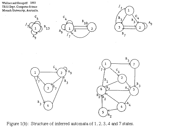
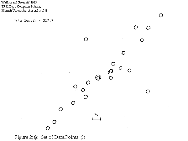
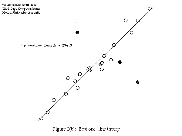
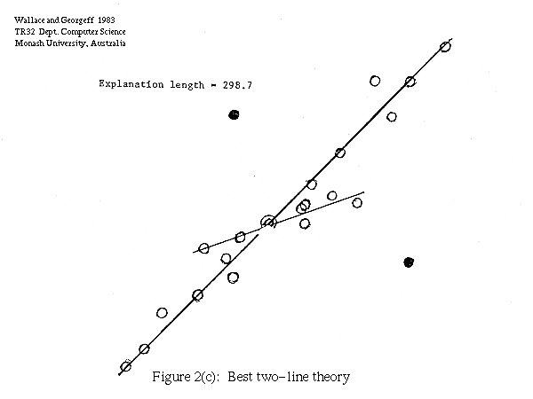
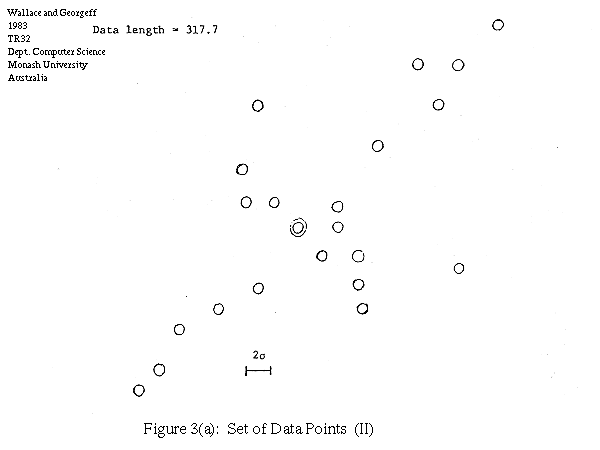
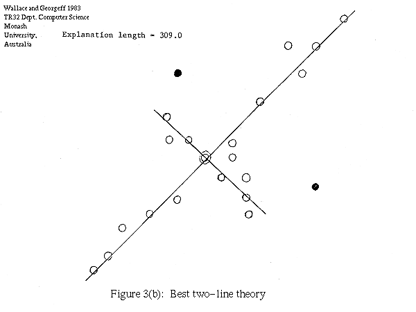
Figure 3(b): Best two-line theory

[This completes TR32, the original printed copy running to 18 pages. Note, the original used the notation lg(x), rather than len(x) as here, for lengths.]

A derived and abridged paper later appeared as:

M. P. Georgeff & C. S. Wallace. A General Selection Criterion for Inductive Inference, European Conference on Artificial Intelligence (ECAI, ECAI84), Pisa, pp473-482, September 1984.

Some Further Reading:

• J. D. Patrick & C. S. Wallace. Stone Circle Geometries: An Information Theory Approach. In Archaeoastronomy in the New World D. Heggie (ed), C.U.P., 1982.
• C. S. Wallace & P. R. Freeman. Estimation and Inference by Compact Coding. J. Royal Stat. Soc. B 49(3), pp240-265, 1987.
• C. S. Wallace. MML Inference of Predictive Trees, Graphs and Nets. In Computational Learning and Probabilitic Reasoning, A. Gammerman (ed), Wiley, pp43-66. 1996.
• M. Viswanathan & C. S. Wallace. A Note on the Comparison of Polynomial Selection Methods. Proc 7th Int. Workshop on Artificial Intelligence and Stats. Ft. Lauderdale, pp169-177, Jan 1999.
• C. S. Wallace & D. Dowe. Minimum Message Length and Kolmogorov Complexity. The Computer Journal, 42(4), pp270-283, 1999
  - In a special issue on Kolmogorov complexity / minimum length encoding methods. The issue also contained other related papers, commentaries on the paper by other authors, and a reply pp345-347. .
• [Chris Wallace's publications]
• [Hidden Markov models].

9/1999: HTML and added mistakes by Lloyd Allison.