Hidden Markov Models

Markov Models

A Markov model is a probabilistic process over a finite set, {S₁, ..., S_k}, usually called its states. Each state-transition generates a character from the alphabet of the process. We are interested in matters such as the probability of a given state coming up next, pr(x_t=S_i), and this may depend on the prior history to t-1.

In computing, such processes, if they are reasonably complex and interesting, are usually called Probabilistic Finite State Automata (PFSA) or Probabilistic Finite State Machines (PFSM) because of their close links to deterministic and non-deterministic finite state automata as used in formal language theory.

Examples are (hidden) Markov Models of biased coins and dice, formal languages, the weather, etc.; Markov models and Hidden Markov Models (HMM) are used in Bioinformatics to model DNA and protein sequences.

Order 0 Markov Models

An order 0 Markov model has no "memory": pr(x_t = S_i) = pr(x_t' = S_i), for all points t and t' in a sequence.

An order 0 Markov model is equivalent to a multinomial probability distribution. The issue of the accuracy with which the model's parameters should be stated, and hence the model's complexity, was investigated by Wallace and Boulton (1968, appendix).

Order 1 Markov Models

An order 1 (first-order) Markov model has a memory of size 1. It is defined by a table of probabilities pr(x_t=S_i | x_t-1=S_j), for i = 1..k & j = 1..k. You can think of this as k  order 0  Markov models, one for each S_j.

Order m Markov Models

The order of a Markov model of fixed order, is the length of the history or context upon which the probabilities of the possible values of the next state depend. For example, the next state of an order 2 (second-order) Markov Model depends upon the two previous states.

Example

Biased Coins

A large biased coin, `A', is described by the order 0 Markov model pr(H)=0.6, pr(T)=0.4.

A small biased coin, `B', pr(h)=0.3, pr(t)=0.7.

A third biased coin, 'C', pr(H)=0.8, pr(T)=0.2.

3 Coins

Consider the following process:

1. Let X equal one of the coins `A' or `B' (above).
2. repeat
   1. Throw the coin X and write down the result.
   2. Toss coin `C'.
   3. if `C' shows T then change X to the other one of {`A',`B'}, otherwise leave X unchanged.
3. until enough

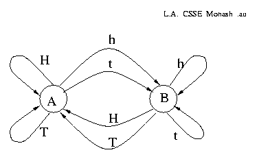
We get the following first-order Markov model over {H,T,h,t}:

	xt-1
	H	T	h	t
pr(xt=H)	0.6×0.8	0.4×0.8	0.3×0.2	0.7×0.2
pr(xt=T)	0.6×0.8	0.4×0.8	0.3×0.2	0.7×0.2
pr(xt=h)	0.6×0.2	0.4×0.2	0.3×0.8	0.7×0.8
pr(xt=t)	0.6×0.2	0.4×0.2	0.3×0.8	0.7×0.8

Below: The process can be drawn as a diagram of states (nodes) and transitions (edges), which makes it clear that it is equivalent to a finite state machine with probabilities associated with each transition:

The probabilities on the arcs out of a given state must sum to 1.

e.g. output HTHHTHHttthtttHHTHHHHtthtthttht...

Hidden Markov Models

A Hidden Markov Model (HMM) is simply a Markov Model in which the states are hidden. For example, suppose we only had the sequence of throws from the 3-coin example above, and that the upper-case v. lower-case information had been lost.

HTHHTHHTTTHTTTHHTHHHHTTHTTHTTHT...

We can never be absolutely sure which coin was used at a given point in the sequence but we can calculate the probability.

Variations

The are a number of variations on HMM problems, e.g.

1. The number of states and transition probabilities are known
   • Given data, find the optimum (most likely) position of the change points;
     this is sometimes called the `segmentation problem' or the `cut-point problem'.
   • How precisely should the points be stated?
   • In some problems the run-lengths of the use of a component model (i.e. one of the coins `A' or `B' above) is generalised and modelled by some appropriate probability distribution.
2. The number of states is known, but the transition probabilities are not
   • Estimate the transition probabilities.
   • What accuracy is appropriate for the estimates?
3. The number of states, and the architecture, are unknown.
   • Find a HMM / automaton which models the data "well".
   • The simplest model has one state, the most complex model has one state per data value; almost certainly neither extreme is justified. Quantifying model complexity is therefore a crucial issue.
   • NB. The cut-point positions are nuisance parameters for this problem.

Automata (Variable Order)

A probabilistic finite state automaton consists of states (drawn as nodes) and transitions (arcs, edges). Each transition causes a character to be output. The automaton moves from state to state outputing characters from its alphabet. Each state can be thought of as an order 0 Markov model, i.e. a multinomial probability distribution, over its outgoing transitions. On the other hand, two or more states may have outgoing transitions labelled with the same set of characters but having different probability distributions. The paths into such states can be thought of as contexts of varying lengths which govern the probability distribution of the character to be output next.

Example

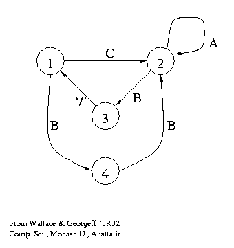
Above: The best probabilistic finite state automaton, in terms of model complexity and fit to the data, for the data  `CAAAB/ BBAAB/ CAAB/ BBAB/ CAB/ BBB/ CB'.  The character `/' is a delimiter, known a priori to cause a return to the start state. The problem was posed by Gaines (1976), the solution is from [TR32] (1983).

The examples start with C or BB, then there are a few A's, and finally B/. The solution shows this. The probabilities of the transitions can be estimated from the observed frequencies.

Inference

If the state transitions of the automaton are known, all that remains is to infer the probabilities of the transitions out of each state, which can be done using the observed transition frequencies (counting).

Sometimes the architecture of the model and the sequence of output characters are known, but not the sequence of state transitions.

In general, neither the architecture of the automaton nor the transitions are known - they are hidden. One must search for an automaton that explains the data well. It is necessary to weigh the trade-off between the complexity of the model and its fit to the data.

Applications

MML and (hidden) finite state models have be used to:

• Infer the grammar of simple languages:
  • C. S. Wallace & M. P. Georgeff. A General Objective for Inductive Inference. [TR32 (HTML)], March 1983, Department of Computer Science, Monash University, Australia.
    Also:
    M. P. Georgeff & C. S. Wallace. A General Selection Criterion for Inductive Inference. European Conference on Artificial Intelligence (ECAI, ECAI84), Pisa, pp.473-482, September 1984.
• Infer the class structure in a time-series or other sequence of multivariate data:
  • T. Edgoose, L. Allison & D. L. Dowe. An MML classification of protein structure that knows about angles and sequence. Pacific Symposium on Biocomputing '98, pp.585-596, Jan. 1998 [paper]
  • T. Edgoose & L. Allison. Minimum message length hidden Markov modelling. IEEE Data Compression Conf., Snowbird UT, pp.169-178, March 1998
  • T. Edgoose & L. Allison. MML Markov classification of sequential data. Stats. and Comp. 9(4) pp.269-278, Sept. 1999
• Model the relationship between pairs of DNA sequences:
  
  • L.Allison, C.S.Wallace and C.N.Yee. Inductive Inference over Macro - Molecules. [90/148], CSSE, Monash University, 1990
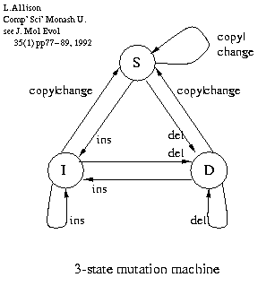
  • L.Allison, C.S.Wallace & C.N.Yee. Finite-State Models in the Alignment of Macro - Molecules. J.Molec.Evol. 35(1) pp.77-89, 1992
  • L.Allison. Normalization of Affine Gap Costs Used in Optimal Sequence Alignment. J.Theor.Biol. 161 pp.263-269, 1993 [www inc' pdf paper]
  • C. N. Yee & L. Allison. Reconstruction of Strings Past. CABIOS 9(1) pp.1-7 (now J. Bioinformatics) 1993
• Align pairs of sequences where each sequence is non-random, e.g. modelled by a finite-state model, or by any "left to right" model:
  
  • D. R. Powell, L. Allison, T. I. Dix, D. L. Dowe. Alignment of low information sequences. Australian Comp. Sci. Theory Symp. (CATS98), Perth, pp.215-230, Springer Verlag isbn:981-3083-92-1, Feb. 1998
  • L.Allison. Information-Theoretic Sequence Alignment. [98/14 (HTML)] CSSE Monash University, 1998
  • L. Allison, D. Powell & T. I. Dix. Compression and Approximate Matching, Computer Journal, 42(1), pp.1-10, 1999
  • D. R. Powell, L. Allison, T. I. Dix. Modelling-Alignment for Non-Random Sequences, AI2004, Springer Verlag, LNCS/LNAI 3339, pp.203-214, Dec. 2004
• Model the relationship between several sequences given an evolutionary (phylogenetic) tree:
  
  • L. Allison and C. S. Wallace. The Posterior Probability Distribution of Alignments and its Application to Estimation of Evolutionary Trees and Optimisation of Multiple Alignments. Jrnl. Molec. Evol. 39 pp.418-430, 1994
• Discover weak and approximate patterns in DNA sequences:
  
  • L. Allison, T. Edgoose, T. I. Dix. Compression of Strings with Approximate Repeats. Intelligent Systems in Molecular Biology ISMB98 pp.8-16, Montreal, 28 June - 1 July 1998
  • L. Allison, L. Stern, T. Edgoose & T. I. Dix. Sequence Complexity for Biological Sequence Analysis. Computers and Chemistry 24(1), pp.43-55, Jan. 2000
  • L. Stern, L. Allison, R. L. Coppel, T. I. Dix. Discovering patterns in Plasmodium falciparum genomic DNA. Molecular and Biochemical Parasitology, 118(2) pp.175-186, 2001
• See MML, Bioinformatics