A Decision Graph Explanation of Protein Secondary Structure Prediction
26th Hawaii International Conference on Systems Sciences (HICSS26), Vol 1, pp.669-678, January 1993
David L. Dowe,
Jonathan Oliver,
Trevor I. Dix,
Lloyd Allison,
Christopher S. Wallace
Department of Computer Science,
Monash University,
Clayton, 3168, AUSTRALIA.
Supported by Australian Research Council grant A49030439.
Oliver and Wallace recently introduced the machine-learning technique of decision graphs, a generalisation of decision trees. Here it is applied to the prediction of protein secondary structure to infer a theory for this problem. The resulting decision graph provides both a prediction method and, perhaps more interestingly, an explanation for the problem. Many decision graphs are possible for the problem; a particular graph is just one theory or hypothesis of secondary structure formation. Minimum message length encoding is used to judge the quality of different theories. It is a general technique of inductive inference and is resistant to learning the noise in the training data.
The method was applied to 75 sequences from non-homologous proteins comprising 13K amino acids. The predictive accuracy for 3 states (Extended, Helix, Other) is in the range achieved by current methods. Many believe this is close to the limit for methods based on only local information. However, a decision graph is an explanation of a phenomenon. This contrasts with some other predictive techniques which are more "opaque". The reason for a prediction can be of more value than the prediction itself.
1. Introduction
A protein is a large and complex molecule consisting of one or more chains. Each chain consists of a back-bone, (N-Calpha-C)+, with one of the 20 possible side-chains (table 1) attached to each alpha-carbon atom, Calpha. The 3-dimensional, folded shape of the protein is responsible for much of its biochemical activity and the prediction of this shape from the primary sequence of the protein is a major, long-term goal of computing for molecular biology. There are several surveys of progress towards solving the problem[27, 25, 30, 23]. Techniques that have been applied include energy minimisation and molecular dynamics[2], statistical methods[7] and artificial intelligence methods[15].
Different levels of protein structure have been recognised[26]:
- aggregate of chains,
- tertiary (3-D) structure of a chain,
- domain, a globular clump of a chain,
- super-secondary structure, arrangement of a "few" secondary structures,
- secondary structure, local structure: helix, extended, turn, coil,
- primary (amino acid) sequence.
It must be said that the boundaries between some of these levels can be blurred. Today it is relatively easy to find the primary sequence of a protein but the full 3-D structure can only be obtained by x-ray crystallography which is both difficult and time-consuming; nuclear magnetic resonance spectroscopy can also provide 3-D information. Many primary sequences but relatively few 3-D structures are known. Certain local or secondary structures recur in proteins: helices, turns, and extended strands which can form beta-sheets. Reliably predicting secondary structure from primary sequence would reduce the 3-D prediction problem from arranging or packing hundreds of amino-acids to packing tens of secondary structures. This explains the considerable interest in secondary structure prediction. Current methods achieve success rates in the 55%[12] to 65%[6] range for 3 states - extended (E), helix(H) and other(O) - on arbitrary proteins. Many believe this to be close to the limit for methods that ignore long-range factors and that use only local information or interactions. It should also be noted that restricting the type of proteins, or using other information - for example the known structure of a protein with a similar primary sequence, if there is one - can much improve predictions.
 1  A  Alanine       Ala
 2  C  Cysteine      Cys
 3  D  Aspartate     Asp
 4  E  Glutamate     Glu
 5  F  Phenylalanine Phe
 6  G  Glycine       Gly
 7  H  Histidine     His
 8  I  Isoleucine    Ile
 9  K  Lysine        Lys
10  L  Leucine       Leu
11  M  Methionine    Met
12  N  Asparagine    Asn
13  P  Proline       Pro
14  Q  Glutamine     Gln
15  R  Arginine      Arg
16  S  Serine        Ser
17  T  Threonine     Thr
18  V  Valine        Val
19  W  Tryptophan    Trp
20  Y  Tyrosine      Tyr
Table 1: Amino Acid Codes.
We use a machine-learning program to infer a decision graph[19, 20] for predicting secondary structure from primary sequence. The main database is that used by a recent version of the Garnier, Osguthorpe and Robson method[7, 8] as incorporated in the Protean II protein analysis package[21]. It consists of 75 protein sequences of known structure. (Earlier work[5] used a set of 50 proteins.) Three states are used, (E,H,O). The resulting decision graph embodies rules that have been inferred from the training data, to assign states. The graph or the rules can then be used to predict states for new proteins. Decision graphs are a generalisation of the well-known decision trees[22]. Graphs have certain advantages over trees including being able to deal with high arity attributes, such as amino acids, more effectively. Section 2 introduces graphs and trees. Logical rules containing conjunction and disjunction are naturally derived from a graph. The rules are probabilistic and indicate a degree of confidence in a prediction. The more confident predictions tend to be more accurate[5]. The graph is a theory or hypothesis about structure prediction. The graph or rules can be taken as an explanation and can be as important as the predictions that are made. A second graph is used to model the serial correlation in secondary structure and to smooth the predictions of the first graph.
Many decision graphs are possible for the secondary structure problem. Minimum message length (MML) encoding is used as the criterion to guide the search for a good graph. A particular graph is (just) a theory or hypothesis. A good graph will predict the data well but a complex graph might be fitting the idiosyncrasies[10] or noise in the training data. Under the MML principle, there is a larger overhead for a complex graph than for a simple one - it must pay its way. This is a computational version of Occam's razor and balances the trade-off in graph complexity. It is described in more detail in section 3.
We believe that the MML criterion is the best yardstick on which to compare methods, whether based on information theory or not, but it is not common practice and so we also give the percentage of correct predictions for comparison purposes. Most experiments reported here used a window of size 7. The data was divided into training and test-sets in various ways. The average success rate for 3 states was 49% to 60%, averaging 55.6%, which is in the typical range for prediction methods, at the lower end.
Many approaches have been taken to computer prediction of secondary structure. There are reviews by Kabsch and Sander[12] in 1983, Schulz[26] in 1988 and Garnier and Levin[6] in 1991. Some of the difficulties in comparing different methods are that standard data-sets are rarely used and that entries in the structure database are "improved" and even deleted.
The Chou-Fasman method[4] is one of the earliest methods and was initially carried out by hand. It is based on coefficients for each pair <a:amino-acid, s:state>, which are derived from the probability of `a' being in state `s' in known structures. Given a new protein, the coefficients are averaged over a small neighbourhood of each position to give a weight to each possible prediction. This does not have a firm statistical justification. Lim[16] gave another early method, based on hand-crafted rules. It performed rather well on the small set of proteins available initially but did not generalise well as more structures became known.
Garnier, Osguthorpe and Robson defined a fully algorithmic and objective method based on information theory and now known as the GOR method[7]. For each triple, <a:amino-acid, p:position, s:state>, a coefficient is calculated from the training data. This is the -log odds-ratio of the central amino-acid in a window being in state `s' against its not being in state `s'. It is calculated for all states `s', amino-acids `a' and positions `p' from -8 to +8 within a window of width 17. To make a prediction, the coefficients are summed over the amino acids in an actual window and this is done for each possible state. (This is equivalent to multiplying the odds-ratios and then taking the -log.) The prediction is for the state having the largest total. The GOR method therefore has sound statistical credentials and is based on a simple but explicit model: that each amino acid in the window makes an independent contribution to the probability of the central amino acid being in a given state. Attempts to take pair-wise interactions into account are hampered by the small size of the structure data base[9].
Neural-nets have been applied to secondary structure prediction[10]. A typical neural-net fits a simple non-linear (sigmoidal) model to the data. The GOR method fits a linear model on -log odds-ratios, so one might expect a neural net to perform similarly, as is the case. On the other hand it is difficult to extract an explicit model from a neural-net to provide an explanation of how the predictions are made.
King and Sternberg[13] devised a system to learn a class of prediction rules automatically. Each rule specified a pattern, being a sequence of amino acids or classes of amino acids.
Muggleton et al[17, 18] have applied Golem to secondary structure prediction. Golem is a general system to infer predicate-logic rules from examples. The rules are in Horn-clause form, essentially a Prolog program. These rules must express disjunction indirectly but otherwise are similar in general form to those created from decision graphs. Unfortunately, the application of Golem was to a restricted set of alpha domain type proteins, making direct comparison with other methods difficult.
The consensus is that the GOR and several other methods can achieve 60-odd% accuracy on arbitrary proteins while the methods of Chou and Fasman and of Lim are less accurate[6]. Higher accuracy is possible in restricted sets of proteins or by using other information. The GOR method is based on a simple, explicit, probabilistic model. Logical rules, created by an expert or inferred by Golem or embodied in a decision graph, are in a general or universal language and can be said to be more of an explanation in the everyday sense.
2. Decision Trees and Graphs
Oliver and Wallace[19] recently introduced the notion of a decision graph which is a generalisation of the well-known decision tree[22]. A decision function is a mapping from a vector of attributes of a "thing" to the class of the thing, eg. from the amino acids within a window to the state of the central amino acid in the window. Decision trees and graphs represent the same class of decision functions but graphs are more efficient in learning rules with a disjunctive nature. This can variously be taken to mean that (for such cases): a graph is learned more quickly on less data, graphs are more expressive or a graph is a more succinct theory.
As an example, consider things having 4 binary attributes, @1 to @4. There are 2 classes, #1 and #2. A thing is in class #1 if @1 and @2 are true or if @3 and @4 are true, otherwise it is in class #2.
A decision tree (figure 1) contains decision nodes and leaves. A decision node specifies a test on an attribute of a thing. The test can be a k-way split on a discrete value or can be an inequality on a continuous value. A leaf node assigns a class to things. The assignment can be probabilistic[33] and can indicate a degree of confidence. To use a tree to predict the class of a given thing, a path is traced from the root of the tree to a leaf following arcs as indicated by the results of tests. A path in a tree represents a conjunction of tests: p&q&r&... . For example, the thing <T,F,T,T> is in class #1 because starting at the root the following directions are taken: left, right, left, left. The resulting leaf predicts class #1.
-
function to be learned:
   class #1 = (@1 & @2) or (@3 & @4)
   class #2 = ~ #1
   binary attributes @1, @2, @3 and @4.
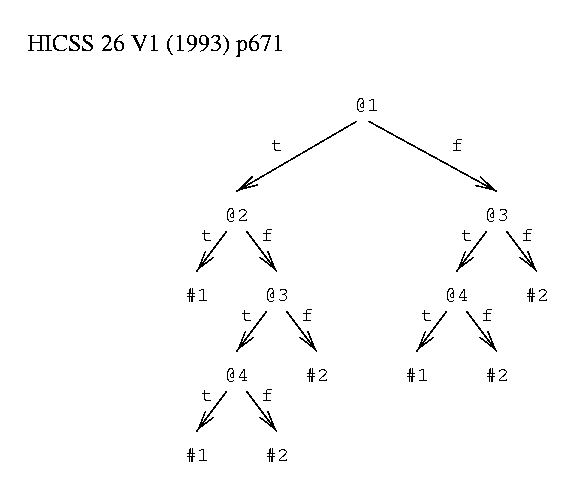
Figure 1: Example Decision Tree.
A decision graph (figure 2) can contain join nodes in addition to decision nodes and leaves. A join node represents the disjunction of the paths leading to it: p or q or r or ... . For example, the sets of things matching <T,F,?,?> and <F,?,?,?> lead to the same join node. This does not add to the class of decision functions that can be described but it does make it much more efficient to describe a wide class of functions.
-
function to be learned:
   class #1 = (@1 & @2) or (@3 & @4)
   class #2 = ~ #1
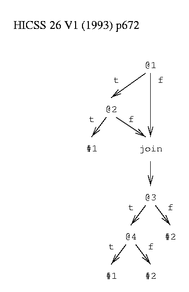
Figure 2: Example Decision Graph.
The most obvious attributes in secondary structure prediction are the amino acids in a window but 20 is a very high arity or fan-out for an attribute. A decision node divides the training data into 20 subsets. 2 levels of decision nodes divide it into 400 subsets. This rapidly halts progress in the inference of a decision tree. On the other hand, decision graphs can delay this problem by joining paths with related outcomes, by adding the data flowing along these paths, and learning a richer theory. (We actually use a 21st pseudo amino acid to indicate "end of chain".) Note, it is also possible to add redundant attributes, possibly with lower arity such as classes that amino acids belong to, but that is not considered here.
There are a great many possible decision graphs for secondary structure prediction. Minimum message length (MML) encoding is used to evaluate graphs and to guide the search for a "good" one. The search can be difficult and lookahead and heuristics are necessary. A greedy algorithm is used with a specified amount of lookahead. Global optimality cannot generally be guaranteed in feasible time. However, any two graphs can be compared with confidence.
3. Minimum Message Length Encoding
Minimum message length (MML) encoding is a general information-theoretic principle[3]. Given data D we wish to infer an hypothesis H. In general there are many possible hypotheses and we can only speak of better or worse hypotheses. Imagine a transmitter who must send a message containing the data to a receiver who is a considerable distance away. If the transmitter can infer a good hypothesis it can be used to compress the data. However any details of the hypothesis that the receiver does not already know, ie. that are not common knowledge, must be included in the message or it will not be comprehensible. The message paradigm keeps us honest - nothing can be passed under the table. We therefore consider two-part messages, which transmit first an hypothesis H and then transmit D using a code which would be optimal if the hypothesis were true. From information-theory, the message length (ML) in an optimal code of an event E of probability P(E) is -log2(P(E)) bits. Therefore the best hypothesis is the one giving the shortest total message.
  ML(E) = -log2(P(E)),
  where event E has probability P(E).

  Bayes' theorem:
   P(H&D)= P(D).P(H|D) = P(H).P(D|H)
  ML(H&D)=ML(D)+ML(H|D)=ML(H)+ML(D|H)

  posterior log odds-ratio:
  -log2(P(H|D)/P(H'|D))
  = ML(H|D)-ML(H'|D)
  = (ML(H)+ML(D|H)) - (ML(H')+ML(D|H'))

  for hypotheses H and H', data D.
P(D|H) is the likelihood of the hypothesis - actually a function of the data given the hypothesis. P(H) is the prior probability of hypothesis H. Oliver and Wallace[19] discuss a prior probablity distribution for decision graphs. P(H|D) is the posterior probability of hypothesis H. The posterior odds-ratio of two hypotheses H and H' can be calculated from the difference in total message lengths: the better one gives the shortest message. The raw data itself constitutes a null-theory and gives an hypothesis test: any hypothesis that gives an overall message length longer than that of the null-theory is not acceptable.
The MML principle has been successfully applied to clustering or classification[31, 32], decision trees[22, 33], decision graphs[19, 20], string alignment[1] and other problems.
Our present decision graphs are hypotheses of secondary structure formation. A graph makes probabilistic predictions of structure. If they are good predictions then the states (E,H,O) can be transmitted very cheaply. Balancing this saving is the cost of transmitting the graph itself. Thus, simple and complex graphs are compared fairly. This prevents the fitting of noise in training data. Some learning techniques tend to generate more complex models given more data. This is not necessarily the case with MML encoding. Certainly small data-sets only justify simple models but large data-sets do not necessarily justify complex models unless there is genuine structure in the data.
4. Methods
4.1 Data
The main database used in our experiments consists of 75 sequences from non-homologous proteins as used in a recent version[21] of the GOR method[7, 8]. The list is given in table 2.
Test-Sets
  1	carbanhy cpase flavodox g3pdh lysot4 ovomucod
	plipase rubredox tim (Size 1687)
  2	adkinase app catalase cona dhfr glucagon
	neurotxb pti staphnuc (Size 1426)
  3	bencejig bencejpr cobratox crambin elastase lysohen
	papainhy plastocy prealb subtilhy superoxd
	(Size 1569)
  4	actinhyd arabbind cytb5 cytb562 cytc cytc550
	cytc551 fecytc2 pglycmut rhodnese (Size 1676)
  5	alph azurin ferredpa ferredsp hbchiron hbhorse1
	hbhorse2 hbhuman1 hbhuman2 hblampry hipip
	myoglob (Size 1583)
  6	adh asptc1 asptc2 chymoch2 chymocow ldh melittin
	protasea (Size 1617)
  7	betatryp cabindpv glutred leghb malatedh rnasech2
	rnasecow thermoly (Size 1717)
  8	aprot2ap aprothyd aprotpen fab1 fab2 insulin1
	insulin2 subinhib (Size 1557)

Training set is the complement of the test-set in each case.
Table 2: Proteins Used.
A window of size 7 was used in the main experiments. This gives reasonable predictions and infers a rich graph - and one that can be presented on a page. Windows of size 5 and 9 gave marginally worse results. Windows of size 1 and 3 gave worse results and large windows could not be justified in MML terms. The window was slid along each protein, the amino acids in the window becoming the attributes, and the state of the central position becoming the class, of a "thing". A 21st pseudo amino acid, denoted by `_', is used to indicate "end of chain".
Decision graphs were derived for the entire database. The parameters controlling the search process were varied to find the best graph, giving the shortest total message length. Additionally, in order to test the predictive power of graphs, the data was divided into various groups. Each group served as a test-set for a graph inferred from a training set which was the union of the other groups. This is perhaps the severest and least biased kind of test of a predictive method - testing on arbitrary proteins when trained on non-homologous proteins.
4.2 Prediction Graph and Rules
Figure 3 shows the decision graph inferred from all 75 sequences using a window size of 7. Attributes or positions are numbered 1 to 7 by the program (rather than -3 to +3), the central, predicted amino acid being at position 4, and this numbering is used in the discussion. Rectangular boxes represent collections of leaf nodes. The observed frequencies of the states, E/H/O, are given in the leaves and at other nodes in the graph. Those at node 1 are for the entire database. The frequencies yield estimates of the probabilities of states[33].
The message length for the graph's structure is 191 bits and for the data given the graph is 17.4 Kbits. The null-hypothesis requires 18.9 Kbits so the graph is statistically significant by a wide margin although we cannot be certain that it is the best possible graph because of the nature of the search process[20].
Study of the graph reveals various groups of amino acids at join nodes. These groups were formed automatically by the program and were not provided as background knowledge. A further possibility to be investigated is to provide these or other groupings or classes in the data to the program as background knowledge so that it could split on attributes of lower arity.
The graphs inferred for different data-sets vary slightly. It is a close thing whether it is better for the top-level test to be on the central amino acid (4), as in figure 3, or on the following one (5). This may be due to proline (P) which is a strong indicator of turns[24]. When a smaller database was used[5], a top-level test on
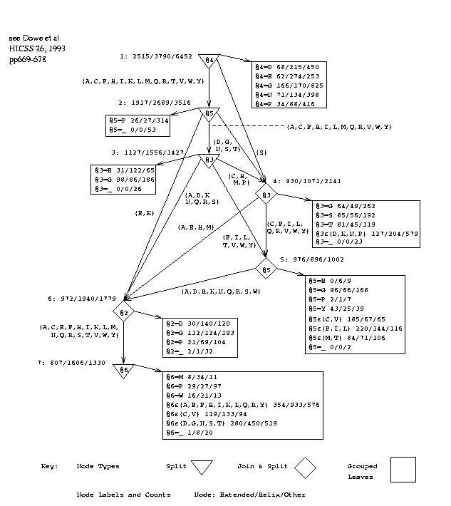 ML(graph) = 191 bits, ML(states|graph) = 17.4 Kbits; Total = 17.6 Kbits ML(null-hypothesis) = 18.9 Kbits Figure 3: Decision Graph, PG, with Window Size 7. |
proline at position 5 led directly to a leaf that was strongly `other', `O', in 270/310 cases. In the current graph, a top-level test on proline at position 4 leads to a leaf that is other in 416/538 cases. A second-level test on proline at position 5 leads to a leaf that is other in 314/367 cases. We also note more tests in the graph that refer to proline and lead to leaves that are strongly other. The earlier graph[5] was based on approximately 8.5K things not directly comparable with the present database. The current graph has fewer decision nodes (7 versus 8) and more join nodes.
The leaves most biased to the extended state in the current graph (figure 3) lie towards the lower right of the graph as children of node 5. There are several paths to these nodes, most of which can be summarised by:
if @4 in [ACFHIKLMQRST  VWY]
 & @3 in [ CF I L    TQRVWY]
 & @5 in [ CF I L       V Y]
then probably extended
We see, for example, that runs of members of [CFILVY] tend to form extended strands. Robson and Suzuki[24, p336] found that these are the 6 strongest indicators of the extended state. They also performed a cluster analysis of amino acids based on secondary structure preferences and reported, "The best defined group is composed of non-polar residues. ... [FILMV]".
The leaves most biased to the helical state lie at the bottom of the graph as children of node 7. Many of the paths here are summarised by:
if @4 in [AC  FHIKLM QR TVWY]
 & @3 in [A DE H K MNQRS    ]
 & @5 in [A DE H K  NQRS  W ]
 & @2 in [AC EFHIKLMNQRSTVWY]
 & @6 in [AC EFHIKLM QR  VWY]
then probably helix
In addition @4=E tends to imply a helix. We conclude that runs of [AEHKQR] tend to form helices. A and E are known to be strong indicators of helices[26]. [EKQH] are close to each other on the codon ring defined by Swanson[28, p155 fig1] where proximity indicates similarity of codons in the genetic code and similarity of physico-chemical properties.
There is an interesting sub-graph of nodes testing positions 3 and 5 in the centre of the graph. With simplification, the paths from node 2 to node 6, the latter of which is biased towards helix, can be approximated by:
   @5 in [EK]
or @3 in [AEHM] & @5 in [DGNST]
or @5 in [ACFHILMQR VWY] & @3 in [AD KNQRS ]
or @3 in [ CF IL QRTVWY] & @5 in [ADHKNQRSW]
[AEM] suggest helix[24] and [DNS] are often at the start of turns, so the second line probably models the transition from a helix to a turn. Note the partial symmetry in lines 3 and 4 between positions 3 and 5 which would be on opposite sides of a helix. The groups on opposite sides in both cases are [CFILQRVWY] and [ADKNQRS]. Taking the differences of these sets gives [CFILVWY] and [ADKNS]. [CFILVY] are non-polar and [ADKNS] are polar which models the tendency of helices to have a hydrophobic side and a hydrophilic side.
The group [DGNST] is formed twice in quite separate parts of the graph although it does not seem to be very strongly biased to one structure. [DGNST] are all `small' and [DNST] are `polar' in Taylor's terms[29]. [DNST] form a leaf-class in a classification of amino acids that Jimenez-Montano derived[11, p653 fig3] from Lim's work[16]. [NST] are members of Robson and Suzuki's ambivalent group[24].
4.3 Smoothing
The above decision graph for secondary structure prediction does not model the serial correlation in secondary structure directly. It may be possible to extend the theory of decision trees and graphs to model series directly, and some alternatives are being investigated, but currently the initial predictions are smoothed by a further decision graph which models just the serial correlation in secondary structure. Two variations of smoothing were tried and others are possible. The first variation is somewhat ad hoc and does not have a simple MML interpretation but it improves the prediction rate by 3.3%. The second variation improves the prediction rate by 2.5% and does have a simple MML interpretation.
4.3.1 Smoothing Variation 1
Figure 4 shows a smoothing graph, SG1, derived from all 75 sequences. The best graph happens to be a tree in this case. Note that the smoothing graph used on a test-set was inferred only from the appropriate training data. The states of the 6 flanking amino acids, positions 1 to 3 and 5 to 7, are the "attributes" of a "thing" and the state of the central amino acid (4) is the "class". This graph models the influence of the flanking states on the central state. When the smoothing graph is created, the actual states of the flanking positions are used as inputs. Each leaf in the graph has pattern(s) associated with it that correspond to the path(s) to the leaf.
The question arises of how to reconcile the possibly conflicting results of the prediction graph `PG' and the smoothing graph `SG1'. The following procedure was
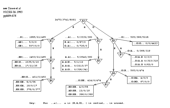 Figure 4: Decision Graph, SG1, Demonstrating Serial Correlation in Conformations. |
used to make a smoothed sequence of predictions for a test protein. Any given sequence of hypothetical states for the protein can be given a probability under PG. To do this the probabilities of the states can be found - from the counts at the leaves of the graph - and multiplied together. Equivalently, the -log probabilities are taken and added, which gives an empirical energy function for the sequence of states under the graph PG. This indicates how consistent the states are with the graph PG.
A similar process is followed for SG1 except that the counts observed in a leaf are used relative to those of the entire training data rather than relative to the total counts within the leaf - this gives more weight to frequent patterns such as ..OOO.. .
The energy is calculated for both PG and SG1 and the results added with a parameter to control the relative weight given to each graph. This ratio was optimised on the training set, being in the range 50:1 to 7:1 and showing that the unsmoothed predictions were fairly sound. A trinomial distribution is derived from the proportions of states (EHO) in the training data. A final term is included in the energy function for the -log probability of the proportion of (predicted) states occuring under the distribution. The search for a sequence of predicted states which minimises the energy function for a given protein was carried out by simulated annealing[14], starting from either the unsmoothed predictions or random predictions.
4.3.2 Smoothing Variation 2
The second method of smoothing used a different decision graph, SG2. SG2 used the 7 predicted states from the prediction graph, PG, as attributes to predict the central state of a window. It can be thought of as a correction graph for PG. Again SG2 was inferred from the appropriate training data. Notionally SG2 was applied simultaneously, in parallel, to all the windows of the entire protein sequence to avoid the question of second-order corrections.
A typical instance of SG2 is quite large and not very interesting. It contains tests that look for isolated predictions of helix, say, which can be over-ridden by their neighbours.
A message length can be calculated for the combined use of PG and SG2. The message would include
                unsmoothed     +SG1        +SG2
       tree      graph PG      graph       graph
set Train Test  Train Test  Train Test  Train Test
--- ----------  ----------  ----------  ----------
 1  55.3  50.8  56.0  54.2  58.8  59.7  58.7  56.5
 2  53.4  50.7  54.0  53.3  56.7  56.7  57.0  57.2
 3  53.1  53.0  54.0  51.7  57.6  58.1  57.2  55.8
 4  54.8  54.3  54.8  56.4  58.4  58.7  58.2  60.3
 5  55.3  42.3  57.9  46.8  61.5  49.5  61.1  48.6
 6  55.0  51.0  55.5  49.0  60.0  49.9  58.6  50.9
 7  54.7  50.1  56.0  52.8  58.2  55.3  57.2  54.7
 8  53.9  53.8  55.3  54.6  57.4  57.0  57.6  54.0
    ----  ----  ----  ----  ----  ----  ----  ----
avg 54.4  50.7  55.4  52.3  58.6  55.6  58.2  54.8

all 55.0   N/A  56.5   N/A  59.7   N/A  58.0   N/A
Table 3: Prediction Success Rates for 3 States.
the structure of PG (191 bits),
- (ii) the predicted state for each leaf of PG (34*log2(3) bits),
- (ii) the structure of SG2 (145 bits) and
- (iv) the cost of the data given PG and SG2 (16.9 Kbits).
- (ii) the structure of SG2 (145 bits) and
SG2 saves about 500 bits on cost of the data alone (part (iv)), over the use of just PG, and the overall saving of about 300 bits is plainly significant.
5. Results
Table 3 gives the success rates for 3 states (E/H/O) on the training data and on the test data for the 8 test-sets, for the prediction graph alone and for the smoothed results. Results are also given for the complete database. (Figures are also given for a decision tree without smoothing.)
The prediction graph alone achieves 56.5% on the full database and an average of 52.3% on the 8 test-sets. The first smoothing method returns 59.7% and 55.6% respectively, and the second smoothing method returns 58.0% and 54.8%. These results are about 2% better than those on the earlier, smaller database[5].
Test-set 5 causes the worst performance on a test set and the best on its training set. This contains several of the globins, and their absence from the training set probably causes the drop in the test-set results relative to the training set results. However the GOR method also performs less well than usual on some of these sequences[8, p449] so perhaps there is something difficult about them.
6. Conclusions
A decision graph is a theory or explanation of secondary structure prediction. The explanation can only be in terms of the information given - here the amino acid sequences. Decision trees are quite familiar in expert systems (a familiar example is in the diagnosis of car faults) and they are generally considered to be comprehensible. A decision graph can be more compact but also more involved, which can be good or bad for purposes of clarity. Logical rules can be extracted from the graph but are likely to be long and numerous if this is done automatically. Muggleton et al[17] noted the difficulty of understanding a large set of logical rules generated by a computer program. To capture the "essence" of a graph in few rules may require simplification and approximation, as in section 4.2, and is not yet an automatic process.
As a prediction method, the performance of the current decision graph is fair. The success rate is in the 49% to 60% range, averaging 55.6% on the test-sets, for a database of 75 sequences and a window of 7. Future work includes giving the decision graph program some background knowledge in terms of amino acid classes, trying both larger databases and restricted classes of proteins, using different window sizes, using a larger number of secondary structure states and investigating different ways of modelling series.
Acknowledgement
Barry Robson very kindly provided the database from the Protean-II package[21].
References
Allison L., C. S. Wallace & C. N. Yee (1992). Finite-state models in the alignment of macro-molecules. J. Mol. Evol. 35(1) 77-89.
Also see [TR90/148(HTML)].Brooks B. R., R. E. Bruccoleri, B. D. Olafson, D. J. States, S. Swaminathan & M. Karplus (1983). CHARMM: a program for macromolecular energy minimization and dynamics calculations. J. Comput. Chem. 4(2) 187-217.
Chaitin G. J. (1966). On the length of programs for computing finite sequences. Jrnl. ACM. 13 547-549.
Chou P. Y. & G. D. Fasman (1974). Prediction of protein conformation. Biochemistry 13 222-245.
Dowe D. L., J. Oliver, L. Allison, T. I. Dix & C. S. Wallace (1992). Learning rules for protein secondary structure prediction. Dept. Res. Conf. 1-12, Dept. Comp. Sci., University of Western Australia; [TR92/163.ps].
Garnier J. & J. M. Levin (1991). The protein structure code: what is its present status. Comp. Appl. BioSci. 7(2) 133-142.
Garnier J., D. J. Osguthorpe & B. Robson (1978). Analysis of the accuracy and implications of simple methods for predicting the secondary structure of globular proteins. J. Mol. Biol. 120 97-120.
Garnier J. & B. Robson (1989). The GOR method of predicting secondary structures in proteins. Prediction of Protein Structure and the Principles of Protein Conformation, G. D. Fasman (ed), Plenum 417-465.
Gibrat J.-F., J. Garnier & B. Robson (1987). Further developments of protein secondary structure prediction using information theory. J. Mol. Biol. 198 425-443.
Holley L. H. & M. Karplus (1989). Protein secondary structure prediction with a neural network. Proc. Natl. Acad. Sci. USA. 86 152-156.
Jiminez-Montano M. A. (1984). On the syntactic structure of protein sequences and the concept of grammar complexity. Bull. Math. Biol. 46(4) 641-659.
Kabsch W. & C. Sander (1983). How good are predictions of protein secondary structure? FEBS Letters 155(2) 179-182.
King R. D. & M. J. E. Sternberg (1990). Machine learning approach for the prediction of protein secondary structure. J. Mol. Biol., 216 441-457.
Kirkpatrick S., C. D. Gelatt jnr. & M. P. Vecchi (1983). Optimization by simulated annealing. Science 220 671-679.
Lathrop R. H., T. A. Webster & T. F. Smith (1987). Ariadne: pattern-directed inference and hierarchical abstraction in protein structure recognition. Commun. ACM. 30(11) 909-921.
Lim V. I. (1974). Algorithms for prediction of alpha-helices and beta-structural regions on globular proteins. J. Mol. Biol. 88 873-894.
Muggleton S., R. D. King & M. J. E. Sternberg (1992). Using logic for protein structure prediction. 25th Hawaii Int. Conf. Sys. Sci. 685-696.
Muggleton S., R. D. King & M. J. E. Sternberg (1992). Protein secondary structure prediction using logic based machine learning. Protein Engineering, to appear.
Oliver J. & C. S. Wallace (1991). Inferring decision graphs. 12th Int. Joint Conf. on Artificial Intelligence (IJCAI), workshop 8, Sydney, Australia.
Oliver J, D. L. Dowe & C. S. Wallace (1992). Inferring decision graphs using the minimum message length principle. Australian Joint Conf. on Artificial Intelligence, Hobart, to appear.
Protean II User Guide. Proteus Molecular Design Limited, Marple, Cheshire, UK (1990).
Quinlan J. R. & R. L. Rivest (1989). Inferring decision trees using the minimum description length principle. Information & Computation 80 227-248.
Reeke jr. G. N. (1988). Protein folding: computational approaches to an exponential-time problem. Ann. Rev. Comput. Sci. 3 59-84.
Robson B. & E. Suzuki (1976). Conformational properties of amino acid residues in globular proteins. J. Mol. Biol. 107 327-356.
Robson B. (1986). The prediction of peptide and protein structure. Practical Protein Chemistry - a Handbook A. Darbre (ed), Wiley 567-607.
Schulz G. E. (1988). A critical evaluation of methods for prediction of protein secondary structures. Ann. Rev. Biophys. Biophys. Chem. 17 1-21.
Sternberg M. J. E. (1983). The analysis and prediction of protein structure. Computing in Biological Science Geisow & Barrett (eds), Elsevier 143-177.
Swanson R. (1984). A unifying concept for the amino acid code. Bull. Math. Biol. 46(2) 187-203.
Taylor W. R. (1986). The classification of amino acid conservation. J. Theor. Biol. 119 205-218.
Taylor W. R. (1987). Protein structure prediction. Nucleic Acid and Protein Sequence Analysis, a Practical Approach M. J. Bishop & C. J. Rawling (eds), IRL Press, 285-322.
Wallace C. S. & D. M. Boulton (1968). An information measure for classification. Comp. J. 11(2) 185-194.
See [HTML].Wallace C. S. (1990). Classification by minimum message length inference. Proc. Int. Conf. on Computing and Information (ICCI), Niagara, Lect. Notes in Comp. Sci 468, Springer-Verlag, 72-81.
Wallace C. S. & J. D. Patrick (1992). Coding Decision trees. Machine Learning, to appear.